A Quantitative Framework for Microservice Decoupling: Balancing Network Latency vs. Domain Boundaries
A mathematically rigorous, production-tested decision framework for balancing microservice decoupling against network latency and consistency penalties.
In high-throughput distributed systems, the road to architectural debt is paved with dogmatic adherence to Domain-Driven Design (DDD) boundaries. Consider a typical production failure: a legacy monolithic checkout operation that historically executed within 35 milliseconds is refactored into a suite of decoupled microservices—Order, Pricing, Tax, Inventory, and Loyalty—to achieve team autonomy and independent deployment. Under moderate load, the p99 latency of the /checkout endpoint balloons to 780 milliseconds. The culprit is not database lock contention or slow SQL queries, but a cascading series of 12 synchronous network hops across the service mesh. Each hop incurs serialization overhead, TLS negotiation, TCP slow-start penalty, and Envoy proxy filter-chain processing. This network amplification depletes downstream worker thread pools, triggers circuit breakers, and causes cascading timeouts. Decoupling code without quantifying the network and consistency penalty is an expensive architectural gamble that often fails in production.
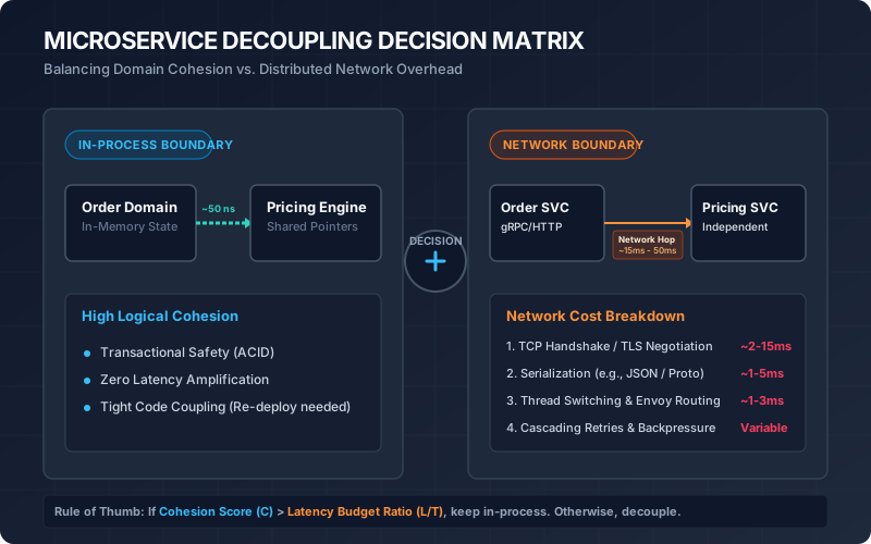
The Hidden Tax of the Network Boundary
When we split a monolithic application into microservices, we replace fast in-memory method invocations with distributed network hops. In-memory calls operate at the nanosecond scale ($10^{-9}$ seconds), passing pointers across stack frames. A network call operates at the millisecond scale ($10^{-3}$ seconds), introducing multiple processing layers:
- System Call and Context Switching: The application must write payloads to a socket, triggering context switches between user space and kernel space. Linux network stack traversal (routing tables, netfilter rules, device driver queues) adds latency before the packet even hits the network interface card (NIC).
- Network Transit: Physical fiber limits transit times. While local VPC network latency within the same cloud availability zone (AZ) is typically sub-millisecond (0.5ms to 1.5ms), cross-AZ transit adds an automatic physical penalty of 1.0ms to 2.5ms per round-trip.
- Proxy Routing and Service Mesh Overhead: In modern Kubernetes deployments utilizing a service mesh like Istio or Linkerd, requests are intercepted by sidecar proxies (Envoy). A single inter-service call goes through egress Envoy processing, network transit, ingress Envoy processing, and finally reaches the target application container. This injects 1.5ms to 4.0ms of latency per hop.
- Serialization and Deserialization: The CPU cost of transforming in-memory objects (e.g., JVM heaps, Go structs) into transport formats (JSON, Protocol Buffers) and back is significant. Under high throughput, garbage collection pauses (JVM GC) and memory allocation overhead during JSON serialization become primary bottlenecks.
| Invocation Type | Transport / Protocol | Payload Size | Typical p99 Latency Overhead |
|---|---|---|---|
| In-Process Call | Memory Pointer | N/A | < 0.001 ms (1 µs) |
| Localhost Loopback | TCP / Unsecured | 10 KB | 0.25 ms – 0.50 ms |
| Inter-VM (Same AZ) | HTTP/2 / gRPC (Proto) | 10 KB | 1.00 ms – 2.50 ms |
| Service Mesh (Envoy mTLS) | HTTP/1.1 / JSON | 100 KB | 4.50 ms – 12.00 ms |
| Cross-Availability Zone | HTTPS / JSON | 100 KB | 6.00 ms – 18.00 ms |
If a single business transaction requires $N$ sequential synchronous calls, the network tax compounds linearly:
\[L_{\text{network}} = \sum_{i=1}^{N} \left( L_{\text{transit}, i} + L_{\text{serialization}, i} + L_{\text{proxy}, i} \right)\]When $N$ exceeds 5, the system enters the danger zone of latency amplification, where minor network fluctuations in any single dependency degrade the p99 response times of the root API.
Defining the Decoupling Trade-Off Index (DTI)
To move beyond gut-feel architecture, we must quantify the decision to split a component. We define the Decoupling Trade-Off Index ($I_d$) as a ratio of domain cohesion to the network latency penalty:
\[I_d = \frac{C_{\text{domain}}}{L_{\text{penalty}} \times F_{\text{call}}}\]Where:
- $C_{\text{domain}}$ is the Domain Cohesion Score ($0 \le C_{\text{domain}} \le 1.0$)
- $L_{\text{penalty}}$ is the Latency Budget Ratio ($0 \le L_{\text{penalty}}$)
- $F_{\text{call}}$ is the Call Frequency Factor (integer $\ge 1$)
1. Calculating Domain Cohesion ($C_{\text{domain}}$)
Domain cohesion evaluates how tightly bound two logical components are from a code and data perspective. It is calculated using two primary metrics: Commit Coupling ($CC$) and Entity Shared Ratio ($ESR$).
Commit Coupling ($CC$): The frequency with which two components are modified in the same version control commit. Using git history over a rolling 180-day window:
\[CC = \frac{|S_A \cap S_B|}{|S_A \cup S_B|}\]where $S_A$ is the set of commits touching component A, and $S_B$ is the set of commits touching component B. A high $CC$ indicates that changes to one domain consistently require changes to the other, pointing to a shared lifecycle.
Entity Shared Ratio ($ESR$): The fraction of domain entities that cross-reference each other or share hard relational database constraints (like foreign keys).
\[ESR = \frac{|E_{\text{shared}}|}{|E_A \cup E_B|}\]where $E_{\text{shared}}$ represents database entities that must be kept transactionally consistent between both domains.
The overall Domain Cohesion Score is defined as a weighted average:
\[C_{\text{domain}} = w_1 \cdot CC + w_2 \cdot ESR\](Recommended defaults in production: $w_1 = 0.6$ for development coupling, $w_2 = 0.4$ for data coupling).
2. Calculating the Latency Budget Ratio ($L_{\text{penalty}}$)
The network latency penalty is relative to the transaction’s overall Service Level Agreement (SLA). If a checkout request must complete in 200ms, a 15ms network hop is manageable. If a payment callback must complete in 20ms, that same 15ms network hop is catastrophic.
\[L_{\text{penalty}} = \frac{\Delta L_{\text{hop}}}{T_{\text{budget}}}\]where $\Delta L_{\text{hop}}$ is the estimated round-trip latency of the proposed network hop (including serialization and sidecar routing) and $T_{\text{budget}}$ is the total latency budget allocated to that specific transaction path.
3. Call Frequency Factor ($F_{\text{call}}$)
$F_{\text{call}}$ represents the average number of synchronous round-trips component A must make to component B to satisfy a single client request. If component A calls component B in a loop for $K$ items, $F_{\text{call}} = K$.
Decision Thresholds for $I_d$
- $I_d > 1.5$ (Strongly Retain In-Process): High domain cohesion coupled with high latency cost. Decoupling will degrade system performance and create a distributed monolith with high coordination overhead. Keep the modules in a single deployment unit (e.g., separate Maven modules, Go packages) and call them in-process.
- $0.5 \le I_d \le 1.5$ (Context-Dependent Evaluative Zone): Decoupling is viable if operational autonomy (e.g., different team scaling, isolated deployment cycles) is critical. Use high-performance RPC protocols (gRPC/Protobuf) to minimize the network tax.
- $I_d < 0.5$ (Strongly Decouple): The domains are highly independent, and the latency budget can easily absorb the network overhead. Decouple into standalone microservices.
Applied Case Study: Checkout vs. Pricing vs. Loyalty
Let’s apply this framework to an e-commerce platform evaluating whether to split its monolithic codebase into three separate microservices: OrderService (Checkout), PricingEngine, and LoyaltyService.
Scenario 1: Splitting PricingEngine from OrderService
During checkout, OrderService must validate items and query PricingEngine to apply dynamic discounts, tax calculations, and volume pricing.
Metrics Gathered:
- Transaction Budget ($T_{\text{budget}}$): 200 ms p99 SLA.
- Estimated Network Hop Latency ($\Delta L_{\text{hop}}$): 12 ms (gRPC over service mesh with mTLS).
- Call Frequency ($F_{\text{call}}$): 3 calls (first for base pricing, second for coupon application, third for final tax validation).
- Commit Coupling ($CC$): Analysis of 250 commits to Order validation shows 110 commits also modified Pricing logic. \(CC = \frac{110}{250} = 0.44\)
- Entity Shared Ratio ($ESR$): The database schema has 5 shared tables (Orders, LineItems, PriceAdjustments, Discounts, Taxes) out of 12 tables total. \(ESR = \frac{5}{12} = 0.417\)
Calculation:
- Domain Cohesion: \(C_{\text{domain}} = (0.6 \times 0.44) + (0.4 \times 0.417) = 0.264 + 0.167 = 0.431\)
- Latency Penalty: \(L_{\text{penalty}} = \frac{12\text{ ms}}{200\text{ ms}} = 0.06\)
- Decoupling Trade-Off Index ($I_d$): \(I_d = \frac{0.431}{0.06 \times 3} = \frac{0.431}{0.18} = 2.39\)
Verdict ($I_d = 2.39$): Keep in-process. The frequency of interaction and domain cohesion are too high to justify a network boundary. Splitting them would result in severe latency amplification ($3 \times 12\text{ms} = 36\text{ms}$ spent on network serialization and routing alone) and high developer friction due to commit coupling.
Scenario 2: Splitting LoyaltyService from OrderService
The LoyaltyService calculates reward points earned on checkout and updates user loyalty tiers.
Metrics Gathered:
- Transaction Budget ($T_{\text{budget}}$): 200 ms p99 SLA.
- Estimated Network Hop Latency ($\Delta L_{\text{hop}}$): 12 ms.
- Call Frequency ($F_{\text{call}}$): 1 call (executed at the end of the transaction).
- Commit Coupling ($CC$): Out of 250 commits, only 10 modified both Order and Loyalty. \(CC = \frac{10}{250} = 0.04\)
- Entity Shared Ratio ($ESR$): The loyalty domain only shares a read-only reference to the Customer ID. \(ESR = \frac{1}{15} = 0.067\)
Calculation:
- Domain Cohesion: \(C_{\text{domain}} = (0.6 \times 0.04) + (0.4 \times 0.067) = 0.024 + 0.0268 = 0.0508\)
- Latency Penalty: \(L_{\text{penalty}} = \frac{12\text{ ms}}{200\text{ ms}} = 0.06\)
- Decoupling Trade-Off Index ($I_d$): \(I_d = \frac{0.0508}{0.06 \times 1} = 0.85\)
Verdict ($I_d = 0.85$): Highly viable for decoupling. The domain cohesion is minimal. Since the lookup can also be optimized as an asynchronous, non-blocking operation post-checkout, the synchronous call frequency factor can be driven to 0 ($F_{\text{call}} \to 0$ in the synchronous path by offloading to an asynchronous message broker like Apache Kafka). This drops the synchronous network penalty to zero.
Production Failure Modes of Decoupling
When engineers ignore quantitative indicators and decouple tightly coupled domains, systems fail in predictable ways:
1. Thread Pool and Socket Exhaustion
In synchronous microservices, blocking HTTP/1.1 client calls hold worker threads open while waiting for downstream responses. If the network experiences a transient latency spike, upstream services queue incoming requests. Under high traffic, this exhausts connection pools and worker thread pools (e.g., Tomcat’s maxThreads or Go’s HTTP goroutines), causing the upstream service to drop connections and crash.
2. The Distributed Transaction Dilemma
In a monolith, updating Order status and reserving Inventory happens within a single database transaction:
-- Monolithic ACID safety
BEGIN TRANSACTION;
UPDATE orders SET status = 'PROCESSING' WHERE id = 123;
UPDATE inventory SET stock = stock - 1 WHERE item_id = 999;
COMMIT;
When decoupled into separate services with separate databases, transactional safety is lost. Engineers must choose between:
- Two-Phase Commit (2PC): A blocking protocol that guarantees consistency but drastically increases latency and introduces deadlocks.
- Saga Pattern (Choreography/Orchestrator): Eventually consistent, but introduces high operational complexity. On inventory failure, compensating transactions must roll back the order. This creates write amplification, where a single action triggers a cascade of writes, event pub/sub cycles, and state checks.
3. Read-After-Write Consistency Anomalies
If a service relies on asynchronous event replication (e.g., using Kafka and Debezium for Change Data Capture) to populate its local read-cache of another domain, there is a replication lag.
[Client] ---> (POST /order) ---> [Order Service] (Writes to DB)
                                        | (CDC Event)
                                        v
                                  [Kafka Broker] (Lag: 250ms)
                                        |
                                        v
[Client] <--- (GET /inventory) <--- [Inventory Service] (Reads stale DB)
If a client writes an order and immediately redirects to the dashboard, they see stale data because the local read model has not caught up. Fixing this requires complex read-through caching strategies or synchronous back-channel verifications, re-introducing the network latency we tried to avoid.
Architectural Mitigation Patterns
If business requirements force the decoupling of components despite a high $I_d$, apply these architectural patterns to minimize the performance penalty:
1. Invert the Query: Data Replication via CDC
Instead of calling a downstream service synchronously over the network for reference data, replicate the data. Use Change Data Capture (CDC) with tools like Debezium and Apache Kafka to stream database updates from the source service to a read-only replica database owned by the calling service.
- Trade-off: You exchange network runtime latency for eventual consistency and local disk storage.
- Application: Ideal for user profile lookup, tax rate tables, and system configurations.
2. High-Performance Transport Tuning
Replace legacy JSON-over-HTTP/1.1 APIs with gRPC over HTTP/2.
- Multiplexing: HTTP/2 allows concurrent requests over a single TCP connection, eliminating head-of-line blocking and reducing TCP handshake overhead.
- Binary Serialization: Protocol Buffers serialize objects to binary format, reducing payload sizes by up to 70% and slashing CPU serialization time compared to JSON parsing.
- TCP Keep-Alives: Configure connection pools to keep TCP sockets warm, preventing connection reuse latency spikes.
# Envoy Proxy Upstream Connection Pool Tuning
upstreams:
  - name: pricing_service
    connection_pool:
      http2:
        max_concurrent_streams: 1024
      common:
        max_connections: 2048
        idle_timeout: 900s
3. Asynchronous Execution (Outbox Pattern)
Never make synchronous network calls to non-critical path dependencies. Use the Transactional Outbox pattern to write events to an local outbox table within the same ACID database transaction, then asynchronously publish them to a message broker.
[Order Service] ---> (ACID Write) ---> [PostgreSQL (Order + Outbox Table)]
                                                  |
                                             (Debezium CDC)
                                                  v
                                            [Kafka Topic]
                                                  |
                                                  v
                                           [Loyalty Service]
This isolates the critical path (checkout) from downstream processing (loyalty points, analytics), keeping the client latency budget intact.
Decision Matrix Checklist
Before decomposing any component, run through this production validation checklist:
- Latent Network Path Analysis: Have you mapped the absolute maximum number of network hops for a single transaction? If $Hops > 4$ for p99 < 150ms, halt decoupling.
- Shared Schema Check: Do the modules write to the same database tables? If yes, resolve the data coupling in-process before attempting to split the network layer.
- Write Cohesion Evaluation: Does a failure in module B require an immediate rollback of module A’s state? If yes, keep them in-process to utilize local transactions rather than distributed Sagas.
- Telemetry Verification: Have you run eBPF tracing (
tcptracerorbpftrace) in your staging environment to measure the exact CPU and network stack processing time of your current boundaries? - Deployment Autonomy Discrepancy: Does team A deploy daily while team B deploys monthly? If yes, this is a strong organizational driver to decouple, but only if the $I_d$ score remains below $1.5$.