Designing a Quantitative Framework for Incident Cost Analysis and Reliability Investment

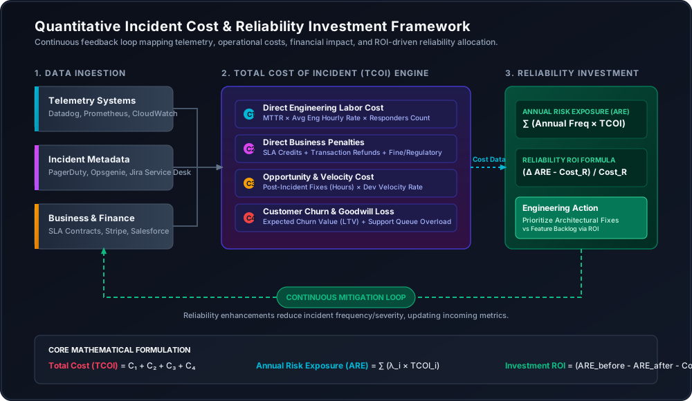
Every engineering lead has sat in a prioritization meeting where a senior engineer pleads for three sprints to refactor a cascading database connection exhaustion issue, only to be shut down by a product manager who needs to ship the Q3 feature roadmap. This deadlock occurs because reliability is discussed in emotional terms—”the system is fragile,” “our pager load is unsustainable”—while feature development is quantified in clear revenue terms. Without a shared mathematical and financial vocabulary, reliability will always lose to features, resulting in a creeping technical debt that eventually manifests as a catastrophic, multi-hour outage. This post designs a quantitative framework that translates backend telemetry, incident response metrics, and contract structures into a loaded financial figure, allowing you to defend reliability investments with the same rigorous ROI math used by the finance team.

The Anatomy of a Hidden Tax: Why Standard Incident Accounting Fails

Standard incident accounting typically stops at basic metrics: Mean Time to Resolution (MTTR), incident volume, and direct billing refunds. If a 30-minute outage on a payment API cost $5,000 in refunds and consumed 10 hours of engineering triage time, a naive spreadsheet will report the incident’s cost as roughly $6,500. This is a microscopic fraction of the true economic damage.

In reality, database lock contention, memory leaks, and third-party API timeouts impose a persistent, hidden tax on engineering organizations. The standard model fails because it ignores several core operational realities:

1. The Context-Switching Tax: Responders do not return to 100% productivity the moment an incident is marked resolved in PagerDuty. The cognitive payload of deep debugging requires a warm-up period. For every hour of active triage, an engineer loses an additional 1.5 to 2 hours of deep-focus work.
2. Post-Incident Drag: The incident doesn’t end when the mitigation script runs. It triggers post-mortem drafting, root-cause analyses (RCAs), cross-team alignment meetings, and high-priority ticket generation. The engineering velocity of the subsequent sprint is directly degraded by these follow-up tasks.
3. Trust Erosion and Churn Lag: A single high-severity outage rarely causes an enterprise customer to cancel their contract immediately. Instead, it places them in a high-risk category. Over the next six months, during contract renewal or upsell discussions, that single incident acts as a leverage point or a silent driver for churn.
4. SLA Cascades: SaaS Service Level Agreements (SLAs) are rarely linear. They operate on threshold cliffs. If your monthly availability SLA is 99.9% and you drop to 99.89%, a contract clause might trigger a flat 10% credit across your entire enterprise client tier, turning a 5-minute blip into a six-figure liability.

To build an objective investment case, we must replace subjective arguments with a repeatable formula: the Total Cost of an Incident (TCOI).

Deconstructing the Total Cost of an Incident (TCOI)

The Total Cost of an Incident ($TCOI$) is the sum of four distinct cost vectors:

Let’s break down the mathematical modeling and operational collection of each component.

C1: Direct Labor Cost (Triage and Mitigation)

This represents the active, loaded engineering cost of diagnosing and mitigating the immediate failure.

Where:

• $R$ is the set of all unique personnel pulled into the incident channel (on-call engineers, secondary responders, engineering managers, customer support reps, and executive communications staff).
• $T_{triage_i}$ and $T_{mitigate_i}$ are the hours spent by responder $i$. This data must be pulled directly from incident management platforms like PagerDuty or FireHydrant.
• $Rate_i$ is the fully loaded hourly rate of employee $i$. A common error is using basic base-salary math. The fully loaded rate must include benefits, equity, and corporate overhead. For a senior backend engineer in the US/EU, this rate is typically between $$150$ and $$250$ per hour.
• $\mu_{fatigue}$ is the Pager Fatigue Multiplier. An incident occurring between 10:00 PM and 6:00 AM carries a multiplier of $1.5$ to $2.0$. This accounts for the downstream productivity drop, sleep deprivation, and operational errors introduced on the subsequent business day.

C2: Direct Financial Impact

This represents the immediate, cash-out-the-door costs associated with the outage.

• $C_{SLA}$: Credits issued due to service level breaches. Calculate this by identifying the percentage of monthly billing that must be refunded per contract terms for the specific downtime duration.
• $C_{refunds}$: Transactions that failed in-flight but were charged, requiring customer support intervention and transaction fee absorption.
• $C_{penalties}$: If processing payments (e.g., Stripe, Adyen) or working with financial networks, outages can trigger chargeback dispute fees (typically $$15$ per dispute) or compliance fines if regulatory reporting thresholds are crossed.

C3: Opportunity and Engineering Velocity Cost

This is the cost of the work the team should have been doing instead of fixing the fallout of the incident.

• $T_{remediation}$: The total engineering hours spent writing the RCA, conducting post-incident reviews, and implementing immediate, non-roadmap bug fixes designed to prevent recurrence.
• $Rate_{team}$: The average fully loaded hourly rate of the engineering team.
• $\eta$: The Developer Velocity Coefficient (a value between 0 and 1 representing the organization’s efficiency). When a team is constantly context-switching to deploy hotfixes, their efficiency drops. We model this drag by calculating the percentage of sprint points carried over or abandoned due to incident remediation.

C4: Reputational Loss and Customer Churn

This is the hardest component to calculate, yet it is often the largest financial driver. We model this as an expected value of risk:

Where:

• $C_{impacted}$ is the set of customers active or affected during the incident.
• $LTV(c)$ is the Lifetime Value of customer $c$.
• $\Delta P_{churn}(c)$ is the marginal increase in the probability of customer churn. This is derived by analyzing historical customer success data. For example, if telemetry shows that enterprise accounts experiencing more than three major outages in a quarter have a churn rate $8\%$ higher than the baseline, then a single outage adds $\Delta P_{churn} = 0.027$ ($8\% / 3$) to that account’s risk profile.

The Math: Defining the Annual Risk Exposure (ARE)

Calculating the cost of past incidents is historical analysis. To justify future investment, we must look forward by defining the Annual Risk Exposure (ARE).

If we have $N$ classified failure modes in our architecture (e.g., database connection pool starvation, memory leaks in the ingestion pipeline, Redis cluster split-brain, or third-party OAuth provider timeouts), we model the ARE as:

Where:

• $\lambda_j$ is the annualized arrival rate (frequency) of failure mode $j$.
• $E[TCOI_j]$ is the expected (average) cost of failure mode $j$.

For high-frequency, low-severity events (e.g., minor Redis CPU spikes), we model $\lambda_j$ using a standard Poisson distribution. For catastrophic “black swan” events (e.g., primary DB corruption), we use extreme value distributions (such as the Gumbel distribution) based on historical industry averages or architectural vulnerability assessments.

Formulating the Reliability ROI

When you propose a reliability initiative (e.g., introducing a caching layer, migrating to a multi-region active-active database, or implementing circuit breakers), you must define the Cost of Prevention ($Cost_R$):

Where $\Delta Cost_{infra_annual}$ is the change in annual cloud infrastructure hosting costs (e.g., upgrading a PostgreSQL RDS instance size or adding read replicas).

The reliability investment is justified if it reduces the Annual Risk Exposure by a delta ($\Delta ARE$) that exceeds the cost of the investment. We define the Reliability ROI ($R_ROI$) as:

Where:

Here, $J$ is the subset of failure modes target-mitigated by the reliability project. If a project completely eliminates a failure mode, $\lambda_{j, mitigated}$ drops to 0. In practice, architectural mitigations rarely eliminate risk entirely; instead, they reduce the arrival rate ($\lambda$) or reduce the severity (MTTR), thereby lowering the expected $TCOI$.

The Decision Rule: If the calculated $R_ROI > 1.5$ (representing a 150% return on engineering capital), the project should be prioritized over new feature work of equivalent engineering cost, unless the product feature carries a verified, short-term revenue generation rate that exceeds the delta risk exposure.

Operationalizing the Framework: Tooling & Instrumentation

You cannot calculate these metrics manually in a spreadsheet every week. You must build an automated ingestion pipeline that aggregates metrics, log states, and financial contracts.

{
  "$schema": "https://json.schemastore.org/geojson.json",
  "incident_id": "INC-8921-A",
  "failure_mode": "postgres_connection_exhaustion",
  "operational_metrics": {
    "start_time": "2026-08-07T02:15:00Z",
    "mitigation_time": "2026-08-07T05:15:00Z",
    "mttr_minutes": 180.0,
    "responders_count": 6,
    "total_responder_hours": 18.0,
    "nighttime_incident": true
  },
  "impact_metrics": {
    "failed_requests": 452000,
    "degraded_requests": 1280000,
    "impacted_tenants_count": 42,
    "impacted_arr": 2400000.00
  },
  "cost_components": {
    "c1_labor_cost": 4050.00,
    "c2_direct_financial": 57000.00,
    "c3_opportunity_cost": 36000.00,
    "c4_expected_churn_cost": 220000.00
  },
  "tcoi": 317050.00
}

Ingestion and Calculation Pipeline

1. Extracting Operational Metrics ($C1$): Use a Cron job or a Webhook listener to poll PagerDuty’s /incidents/{id}/log-entries endpoint. Extract the timestamps for alert trigger, user acknowledgment, delegation, and resolution. Parse the responder user IDs to map them to salary tiers in your HR system (e.g., Workday API). Apply a $1.5\text{x}$ multiplier if the alert trigger timestamp falls outside local business hours ($09:00 - 18:00$).
2. Quantifying Impacted Revenue ($C2$ & $C4$): When an outage is detected, query your APM (e.g., Datadog API) for transactions grouped by client identifier (tenant_id or account_id). Cross-reference the list of degraded or failing client IDs with your billing system (e.g., Stripe API) or CRM (e.g., Salesforce API) to extract the Annual Recurring Revenue (ARR) and specific SLA parameters for those tenants.
3. Storing the Incident Record: Write the parsed and calculated incident records into an internal Postgres database. You can query this database using SQL to build a live dashboard showing the true cost of reliability issues over time.

For example, to find the average cost of incidents by failure mode over the last year:

SELECT 
    failure_mode,
    COUNT(incident_id) AS incident_count,
    ROUND(AVG(tcoi)::numeric, 2) AS avg_tcoi,
    ROUND(SUM(tcoi)::numeric, 2) AS total_annual_cost
FROM incident_costs
WHERE start_time >= NOW() - INTERVAL '1 year'
GROUP BY failure_mode
ORDER BY total_annual_cost DESC;

This SQL output provides the precise numbers needed for the $ARE$ calculation.

A Concrete Case Study: The $320,000 DB Deadlock

Let’s apply this framework to a real incident on a high-throughput SaaS platform processing transactional API payloads.

The Context

A microservice deployment introduced an unindexed foreign key check combined with an nested transaction block on the orders table. Under a peak load of 250 Requests Per Second (RPS), this caused severe row lock contention. The system reached PostgreSQL connection pool saturation (pg pool size = 50), which cascaded upstream, causing timeouts, memory exhaustion in the Node.js API layer, and a complete system lockup.

The Incident Response ($C1$)

• Timeline: The alert fired at 2:15 AM. The primary responder spent 45 minutes digging through Datadog APM and pg_stat_activity to find the blocking lock. They spent another 60 minutes attempting to gracefully terminate the backend transactions. Ultimately, the team had to perform a forced database failover to the replica, causing 5 minutes of total write downtime and 70 minutes of replica lag synchronization. The incident was resolved at 5:15 AM (MTTR = 180 minutes).
• Responders: 4 senior backend engineers, 1 Engineering Manager, and 1 Director of Core Infrastructure.
• Labor Calculation: \(\text{Responders (6)} \times \text{Duration (3 hours)} = 18 \text{ hours}\) Applying the nighttime multiplier ($\mu_{fatigue} = 1.5$) and the average loaded rate ($$150/\text{hr}$): \(C1 = 18 \times \$150 \times 1.5 = \$4,050\)

Direct Financial Impact ($C2$)

• SLA Penalties: 8 enterprise accounts experienced write failures exceeding their monthly downtime allocation of 0.05% (approx 21.6 minutes). The contract clauses triggered a flat 5% credit on their monthly billing. \(\text{Monthly Billing} = \$900,000 \implies C_{SLA} = \$900,000 \times 0.05 = \$45,000\)
• Failed Transactions: 12,000 requests failed mid-flight, forcing manual customer support intervention and refunds. The direct processing fees and refund administrative overhead cost $$1 per ticket: \(C_{refunds} = \$12,000\) \(C2 = \$45,000 + \$12,000 = \$57,000\)

Opportunity & Velocity Cost ($C3$)

• Remediation: Two engineers were pulled off feature development for two weeks (80 hours each) to write the RCA, optimize the index, and split the nested transactions into an asynchronous event queue pattern. \(C3 = 160 \text{ hours} \times \$225/\text{hr (fully loaded)} = \$36,000\)

Reputational Cost ($C4$)

• Customer Churn: Two months after the incident, a high-value customer (ARR = $$220,000$) cancelled their contract, explicitly citing “production instability during Q3” as their primary reason. \(C4 = \$220,000\)

The Total Cost

Adding the components together, the total cost of this database deadlock is:

The Reliability Proposal

The backend team proposed a reliability initiative:

1. PgBouncer Migration: Implement PgBouncer as a connection pooler to prevent client-side connection leaks from crashing the DB.
2. Statement Timeouts: Configure strict statement_timeout (2s) and lock_timeout (1s) at the application adapter level.
3. Lock Alerts: Build Prometheus alerts for pg_stat_database_conflicts and pg_locks queue length.

The Investment Cost ($Cost_R$)

• Engineering Effort: 2 engineers for 4 weeks (160 hours each): \(\text{Labor} = 320 \text{ hours} \times \$150/\text{hr} = \$48,000\)
• Infrastructure Delta: High-availability PgBouncer instances running on AWS ECS: \(\text{Infrastructure Cost} = \$200/\text{month} = \$2,400/\text{year}\) \(Cost_R = \$48,000 + \$2,400 = \$50,400\)

The ROI Calculation

Historical telemetry showed database lock events occurred four times in the past year, with an average $TCOI$ of $$317,050$.

With the proposed statement timeouts and PgBouncer architecture, database connection exhaustion would be mitigated automatically before cascading to upstream services, preventing major downtime. The projected incident frequency ($\lambda$) drops from $4.0$ to $0.2$ per year.

Applying our ROI formula:

An $R_ROI$ of 22.9x is an undeniable business case. Presented with this data, the VP of Product immediately agreed to pause the roadmap for two sprints. The team implemented the changes, and the database has not experienced a cascading outage since.

Addressing Pitfalls and Cognitive Biases

When implementing this framework, you will face pushback and psychological biases from both product and engineering teams:

1. The Sunk Cost Fallacy

“We already spent six months rewriting our API service to use Go; we can’t stop now to fix PostgreSQL locks.” A database rewrite does not fix bad queries. If your framework shows that database locks are responsible for 80% of your $ARE$, you must halt the Go rewrite and fix the schema. The money spent on the Go rewrite is gone; focus engineering capital where the risk reduction is highest.

2. Overestimating Mitigation Success (The “Silver Bullet” Trap)

Engineers tend to assume that their proposed architectural fix will completely eliminate the target failure mode ($\lambda_{mitigated} = 0$). This is almost never true. Assume that any reliability project will reduce the failure rate by a maximum of 80% to 90%. Always budget for a residual risk of 10% when running your ROI calculations.

3. Sandbagging Estimates

To push their favorite technical refactoring projects forward, engineers may artificially inflate the estimated $TCOI$ or underestimate the engineering effort required to implement the fix. To prevent this, the financial metrics (average loaded salaries, customer LTV, SLA terms) must be locked by finance and product operations. The only variables the engineers should control are estimated MTTR reductions and project timelines.

Conclusion

Reliability is not a technical preference; it is a financial constraint. Treating database timeouts and connection pools as aesthetic code quality problems is a recipe for organizational friction. By converting operational telemetry into financial risk exposure, you change the conversation from “we need to clean up technical debt” to “we can prevent $$1.2\text{M}$ in annual losses with a $$50,400$ engineering investment.” This shifts the engineering lead’s role from a petitioner begging for time into a business manager making logical, data-driven investments in the system’s foundation.