A Quantitative Framework for Capacity Planning: Modeling Service Resource Headroom against SLO Violations under Peak Load

It is a scenario familiar to every seasoned on-call engineer: during a highly publicized marketing campaign or a seasonal traffic peak, a critical microservice begins throwing HTTP 504 Gateway Timeout errors. You look at the Grafana dashboard, only to find the CPU utilization hovering at a seemingly safe 70% and memory consumption flat. Because the capacity plan was built around the arbitrary rule of thumb that “30% resource headroom is safe,” the system was assumed to be resilient. Instead, thread pools saturated, garbage collection pauses escalated, and database connection queues blew out, triggering a cascading failure that took down the checkout pipeline. Arbitrary, linear capacity planning rules are not just intellectually lazy; they are a liability in high-throughput production environments because they fail to capture the non-linear relationship between resource utilization and tail latency.

The Fallacy of Linear Headroom Rules

Traditional capacity planning relies on basic arithmetic: if a single service instance handles 1,000 Requests Per Second (RPS) at 50% CPU utilization, we assume it can safely handle 2,000 RPS at 100% CPU. Consequently, we provision instances based on a linear extrapolation, adding a “safety buffer” of 20% or 30%. This approach is fundamentally flawed because computer systems do not scale linearly.

In production, microservices are networks of queues and servers. Thread pools, network sockets, database connection pools, file descriptors, and CPU cores are all resources that requests must compete for. As resource utilization ($\rho$) approaches 100% (or 1.0), the time spent waiting in queues grows hyperbolically, not linearly.

This behavior is described mathematically by Kingman’s formula for queueing delay in a single-server queue ($G/G/1$ approximation):

Where:

• $\rho$ is the resource utilization ($\frac{\lambda}{c \mu}$, where $\lambda$ is the arrival rate, $\mu$ is the service rate, and $c$ is the number of processing cores/threads).
• $C_a^2$ is the squared coefficient of variation of request arrivals (traffic burstiness).
• $C_s^2$ is the squared coefficient of variation of service times (processing complexity variation).
• $\tau$ is the mean service time.

Observe the term $\frac{\rho}{1-\rho}$. As utilization ($\rho$) increases from 0.5 to 0.9, the queueing delay multiplier jumps from 1.0 to 9.0. At 95% utilization, it is 19.0. A small 5% increase in traffic can result in a 200% increase in tail latency.

Furthermore, this queueing behavior is compounded by runtime-specific failure modes:

1. Garbage Collection (GC) Thrashing: In managed runtimes like Go or Java, high allocation rates under load increase GC frequency. Under memory pressure, the JVM’s G1GC or Go’s scavenger spends more CPU cycles reclaiming memory, robbing the application of CPU cycles precisely when throughput is highest. This creates a positive feedback loop: slower request processing leads to more concurrent requests in flight, which increases memory pressure, triggering more GC pauses.
2. Thread Context Switching: When thread pools (like Tomcat’s exec threads or gRPC thread pools) are oversized to compensate for blocking I/O, high load forces the Linux scheduler to constantly swap threads. The CPU spends more time executing kernel-level context switches than doing actual application work.
3. Connection Pool Exhaustion: Databases and external cache layers have strict limits on concurrent connections. Once the pool is exhausted, requests queue inside the application, holding memory and network buffers open, eventually crashing the load balancer with connection resets.

To build a resilient service, we must abandon the “percent CPU headroom” metric and replace it with a quantitative framework that models tail-latency SLO budgets against actual load limits.

Mathematically Modeling Service Saturation: The Knee Point

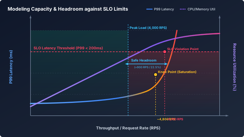
Every system has a “Knee Point”—the throughput threshold where the queueing delay begins to dominate the service time. Beyond this point, the system enters the saturation phase. Our goal is to identify this knee point mathematically rather than waiting to discover it during an active outage.

Let $L(x)$ represent the P99 tail latency of a service as a function of its throughput $x$ (in RPS). In a healthy state, $L(x)$ is relatively flat, dominated by the execution time of the code itself (I/O, serialization, DB queries). As $x$ approaches the physical saturation limit $b$, the latency increases asymptotically.

A robust mathematical model to fit this behavior is a rational function of the form:

Where:

• $L_0$ is the baseline tail latency of the system under zero-load conditions (in milliseconds).
• $b$ is the theoretical maximum throughput (in RPS) where the system fully saturates (the vertical asymptote).
• $a$ is a scaling parameter that represents system sensitivity to load increases.

The Knee Point ($R_{sat}$) is defined as the coordinate where the rate of change of the slope (the second derivative of latency with respect to load) reaches its maximum curvature, or where the system transitions from linear resource consumption to exponential queueing.

To solve for the point of maximum curvature $\kappa(x)$, we use the standard geometric curvature formula:

Determining this point analytically allows us to establish the absolute upper boundary of the “safe operating zone.” Operating any service beyond $R_{sat}$ means that even a minor, temporary 1% spike in traffic will degrade latency to unacceptable levels, rendering autoscaling groups useless because the VM bootstrap time (typically 60–180 seconds) is orders of magnitude slower than the rate of queue saturation (which occurs in milliseconds).

Establishing the SLO-RPS Frontier

While the Knee Point represents the mathematical boundary of system stability, it does not guarantee that we are meeting our business obligations. For this, we must map our tail-latency Service Level Objectives (SLOs) directly onto the load curve.

An SLO is typically defined as:

“The P99 latency of the /checkout endpoint must be less than 200ms over a rolling 5-minute window.”

This threshold is a horizontal line across our latency-load graph. The intersection of this SLO threshold ($L_{SLO}$) and our tail-latency curve $L(x)$ defines the SLO-RPS Frontier ($R_{SLO}$):

Using our rational model, we can solve for $R_{SLO}$:

This equation tells us the maximum throughput a single instance can support before it violates the SLO.

There are two critical scenarios to analyze:

1. $R_{SLO} < R_{sat}$ (Safe Cliff): The SLO threshold is crossed while the system is still operating in its linear range. This is the ideal state. If the load spikes slightly past the SLO frontier, the latency degrades gracefully, giving autoscaling systems or rate-limiters time to react.
2. $R_{SLO} > R_{sat}$ (Dangerous Cliff): The SLO threshold is located past the Knee Point, on the asymptotic vertical section of the curve. This is a highly unstable configuration. Because the curve is nearly vertical at this point, the difference in throughput between satisfying the SLO and total service collapse is negligible (often less than 50 RPS). If your service is configured to run up to this limit, any minor network jitter or database lock contention will cause a massive, immediate SLO violation.

In production, your operational limit must always be bounded by the minimum of these two points:

Calculating Quantitative Headroom and Scaling Factor

With $R_{limit}$ defined for a single instance, we can calculate the required cluster capacity under peak load. Let $R_{peak}$ be the projected peak load for the entire microservice (e.g., during a flash sale).

We define the Load Headroom ($H_{load}$) as the percentage of additional traffic the current deployment can handle before violating our operational limit:

Where:

• $N$ is the number of active, healthy service instances.
• $R_{limit}$ is the per-instance capacity limit derived above.

If $H_{load} \le 0$, the system is under-provisioned and will fail during peak load.

To determine the exact number of instances required to handle a projected peak load while maintaining a target safety headroom factor $S_{target}$ (where $S_{target} = 1 / (1 - H_{load_target})$), we use the following formulation:

Here, we introduce $\phi$, the Systemic Efficiency Multiplier ($0 < \phi \le 1.0$). In a perfect world, load is distributed evenly across all instances, and $\phi = 1.0$. In production, $\phi$ is always less than 1.0 due to several real-world factors:

• Load Balancer Imbalance: Round-robin or least-connections algorithms do not account for request payload size or processing complexity. A single instance may receive a disproportionate number of heavy write requests.
• Routing Topology: gRPC load balancing over HTTP/2 keep-alives often leads to unbalanced connections if clients do not perform periodic subchannel connection draining.
• Database Key Hotness: If your caching layer routes requests based on consistent hashing (e.g., Redis Cluster), a single “hot key” (like a popular merchant or item) will concentrate load onto a single node or instance, causing it to saturate far ahead of the rest of the cluster.

For a standard Kubernetes deployment behind an NGINX Ingress controller, we typically observe a $\phi$ between 0.82 and 0.88. If you run gRPC without a service mesh (like Linkerd or Istio) doing request-level load balancing, $\phi$ can drop as low as 0.65.

Practical Implementation: Load Testing, Profiling, and Continuous Validation

To implement this quantitative framework, you cannot rely on synthetic bench-testing. You must profile your service under simulated production conditions. Here is the operational blueprint for extracting these metrics.

Step 1: Coordinated Omission-Free Load Testing

Using standard load testing tools like ApacheBench or basic wrk can skew your tail latency metrics. These tools suffer from Coordinated Omission: if the server stalls, the tool halts sending new requests, waiting for the active requests to finish. This hides the queueing delay that real users would experience.

Instead, use wrk2 or k6 configured with constant arrival rate execution. The following k6 script executes a stepped load test, ramping throughput to find the saturation point:

import http from 'k6/http';
import { check, sleep } from 'k6';

export const options = {
  scenarios: {
    ramping_arrival_rate: {
      executor: 'ramping-arrival-rate',
      startRate: 100,
      timeUnit: '1s',
      preAllocatedVUs: 500,
      maxVUs: 2000,
      stages: [
        { target: 1000, duration: '5m' }, // Ramp up to 1000 RPS
        { target: 1000, duration: '2m' }, // Hold
        { target: 2000, duration: '5m' }, // Ramp to 2000 RPS
        { target: 2000, duration: '2m' }, // Hold
        { target: 3000, duration: '5m' }, // Ramp to 3000 RPS
        { target: 3000, duration: '2m' }, // Hold
        { target: 4000, duration: '5m' }, // Ramp to 4000 RPS (or crash)
      ],
    },
  },
};

export default function () {
  const res = http.get('http://target-service.local/api/v1/resource');
  check(res, {
    'status is 200': (r) => r.status === 200,
  });
  sleep(0.1);
}

Step 2: Querying Prometheus Metrics

During the load test, extract the throughput and corresponding P99 latency. Run this Prometheus query to get the P99 latency in 1-minute buckets:

histogram_quantile(0.99, sum(rate(http_request_duration_seconds_bucket{job="target-service"}[1m])) by (le))

And query the actual throughput (RPS) handled:

sum(rate(http_requests_total{job="target-service", status="200"}[1m]))

In addition to latency and load, monitor resource utilization metrics. If running in Kubernetes, capture CPU throttling, which occurs when a container exceeds its CFS quota despite reporting low average CPU usage:

sum(rate(container_cpu_cfs_periods_throttled_total{container="target-service"}[1m])) / sum(rate(container_cpu_cfs_periods_total{container="target-service"}[1m])) * 100

If this throttling metric spikes above 5%, the container is CPU-starved during micro-bursts, which will artificially pull the Knee Point to the left.

Step 3: Curve-Fitting with SciPy

Export the Prometheus data points as a CSV containing two columns: RPS and P99_Latency_MS. Use the following Python script to run a non-linear least squares fit to determine your service parameters and compute the SLO frontier:

import numpy as np
import pandas as pd
from scipy.optimize import curve_fit

# Rational model defining latency behavior
def latency_model(x, L0, a, b):
    # x represents throughput in RPS
    # L0 is the base latency
    # b is the theoretical vertical asymptote (physical ceiling)
    # We add a small epsilon to prevent division by zero during optimization
    return L0 + (a * x) / (np.maximum(b - x, 0.001))

# Load your exported metrics
# csv format: rps, p99_ms
data = pd.read_csv("load_test_results.csv")
x_data = data['rps'].to_numpy()
y_data = data['p99_ms'].to_numpy()

# Fit parameters. Set initial guesses (p0):
# L0 ~ minimum observed latency, b ~ maximum tested RPS + 10%
initial_guesses = [y_data.min(), 50.0, x_data.max() * 1.1]

popt, pcov = curve_fit(
    latency_model, 
    x_data, 
    y_data, 
    p0=initial_guesses, 
    bounds=([0.1, 0.01, x_data.max()], [1000.0, 10000.0, x_data.max() * 2])
)

L0, a, b = popt
print(f"--- Fit Results ---")
print(f"Baseline Latency (L0): {L0:.2f} ms")
print(f"Scaling Factor (a):     {a:.4f}")
print(f"Physical Ceiling (b):   {b:.2f} RPS")

# Define our SLO Threshold
SLO_MS = 200.0

if L0 >= SLO_MS:
    raise ValueError("Baseline latency exceeds SLO. Optimize application performance first.")

# Calculate the SLO-RPS Frontier
r_slo = (b * (SLO_MS - L0)) / (a + SLO_MS - L0)
print(f"SLO-RPS Frontier (R_SLO): {r_slo:.2f} RPS at P99 < {SLO_MS}ms")

# Calculate the Knee Point using a heuristic slope change (e.g., derivative = 0.5 ms/RPS)
# For L(x), L'(x) = a*b / (b - x)^2. We find where L'(x) = 0.5 (tangent gradient threshold)
slope_threshold = 0.5
r_knee = b - np.sqrt((a * b) / slope_threshold)
print(f"Calculated Knee Point (R_knee): {r_knee:.2f} RPS")

operational_limit = min(r_slo, r_knee)
print(f"Target Operational Capacity (R_limit): {operational_limit:.2f} RPS")

Step 4: Automating Continuous Capacity Validation

System performance is dynamic. A dependency upgrade, a change in database schema, or a new serialization library can shift your load-latency curve.

1. Integrate load tests into the CI/CD pipeline: Run a headless 10-minute load test in a staging environment cloned from production configuration.
2. Verify regression trends: If a new PR shifts $R_{limit}$ down by more than 10%, break the build or raise an alert. This catches thread lock contention and memory leaks before they reach the main branch.
3. Dynamic Autoscaling Policy: Instead of scaling Kubernetes HPA based on CPU (TargetCPUUtilizationPercentage: 70), scale based on custom Prometheus metrics representing the actual Load Headroom ($H_{load}$). This ensures the cluster scales up before the queueing delays manifest.

apiVersion: autoscaling/v2
kind: HorizontalPodAutoscaler
metadata:
  name: checkout-service-hpa
spec:
  scaleTargetRef:
    apiVersion: apps/v1
    kind: Deployment
    name: checkout-service
  minReplicas: 10
  maxReplicas: 100
  metrics:
  - type: External
    external:
      metric:
        name: service_load_headroom
      target:
        type: Value
        averageValue: "0.25" # Keep load headroom at or above 25%

Summary

Capacity planning is a quantitative discipline, not a guessing game. Operating a high-throughput backend service requires moving away from static utilization rules of thumb and embracing mathematical performance models. By modeling the non-linear relationship between load and latency, pinpointing the queueing knee point, and calculating safety factors that account for load balancing imbalances, we can design architectures that survive peak events. Run the load tests, fit the curves, find your true operational limits, and engineer your headroom.