Designing a Quantitative Framework for Allocating Engineering Capacity between Product Features and Technical Debt

Imagine a Friday evening deployment that should have been routine. Instead, a minor database migration triggers a cascade of lock timeouts, CPU spikes, and API gateway timeouts because the service logic is tangled in a spaghetti codebase. The team spends the weekend firefighting. The root cause? Six months of deferred refactoring on a high-throughput transaction loop to meet product launch deadlines. The classic "negotiation" between product and engineering over technical debt is broken because it relies on gut feelings and emotional pleading. When engineering says "our database query compiler is slow and needs a refactor," product hears "engineers want to play with new technologies instead of building value." To break this deadlock, engineering teams must move away from qualitative arguments and establish a quantitative framework that treats technical debt capacity not as a negotiation, but as a dynamic control system fed by concrete telemetry: code churn, developer loss hours, SLO budget deficits, and deployment failure rates.

The Failure Modes of Qualitative Allocation

Relying on qualitative discussions to allocate engineering capacity is a recipe for operational instability and developer burnout. In most organizations, capacity allocation degenerates into one of three standard failure modes.

1. The Fixed Ratio Fallacy (The “Always 20%” Rule)

Many engineering organizations attempt to solve the capacity problem by decreeing a fixed allocation: 70% product features, 20% technical debt, and 10% maintenance. While simple, this approach fails because it is static. When a product team is chasing an aggressive quarterly milestone, the 20% allocation for technical debt is the first line item to be quietly cut or deprioritized. Conversely, during architectural inflection points—such as a database migration or a major framework upgrade—20% is woefully inadequate. The fixed ratio ignores the shifting reality of the codebase and production environments.

2. Squeaky Wheel Allocation

Without quantitative metrics, capacity is allocated to the engineers who complain the loudest or to the most visible components. This leads to a severe misallocation of resources. For example, a senior developer might spend two weeks refactoring a utility library in a low-traffic service because the formatting bothered them, while a critical connection leak in a high-throughput transaction pool (processing 15,000 RPS) goes ignored because the engineers working on it are less vocal.

3. The Jira Backlog Abyss

Some teams maintain a “Tech Debt Backlog” with hundreds of unprioritized tickets. These tickets collect dust because there is no mechanism to compare the value of a refactoring ticket with the value of a new product feature. Because the backlog is static and disconnected from business outcomes, it becomes a graveyard of good intentions rather than an actionable queue of engineering priorities.

Defining the Metrics: The Input Signals

To build a quantitative framework, we must feed the capacity allocation engine with objective, automated telemetry. We categorize these signals into two main domains: Developer Friction and System Instability.

Developer Loss Hours (LH)

Developer Loss Hours represents the time wasted by engineers due to sub-optimal toolchains, slow CI pipelines, and architectural complexity. This metric is a direct proxy for the “interest rate” of your technical debt.

To calculate this, we aggregate the following telemetry from tools like the GitHub Actions API, Buildkite, and local development helper scripts:

• CI/CD Pipeline Duration ($T_{CI}$): The average time spent waiting for test suites to complete. If a pipeline takes 25 minutes and a developer runs it 4 times a day, they waste 100 minutes daily.
• Local Environment Bootstrap Failures ($F_{env}$): The number of times a developer’s local environment fails to compile or spin up due to config drift, requiring manual intervention.
• Context-Switching Cost: Studies show that it takes an average of 23 minutes to recover focus after a context switch. We model this by applying a multiplier ($1.5\times$) to any CI pipeline wait time exceeding 10 minutes.

The formula for monthly Developer Loss Hours ($LH$) for a team of size $N$ is defined as:

Code Hotspot Index (CHI)

Not all complex code is technical debt. A file containing 1,000 lines of complex legacy Go code that has not been modified in two years is not costing the team money. It is stable. However, a 300-line file that is complex and experiences high code churn is a major bottleneck.

We define the Code Hotspot Index ($CHI$) for each source file as:

• Churn: The number of commits touching the file in the last 30 days.
• Complexity: The cyclomatic complexity (using AST parsers like lizard or SonarQube) or cognitive complexity.

Any file with a $CHI$ score above the 90th percentile of the repository is classified as a “hotspot” and triggers a capacity adjustment.

Service Level Objective (SLO) Deficit

If a service is burning through its error budget, product delivery must slow down to address stability. We pull availability and latency metrics from Prometheus or Datadog and calculate the SLO Deficit ($SLOD$):

If your target P99 latency is $< 200\text{ms}$ at 99.9% availability, and the service is delivering 99.5% availability, the $SLOD$ rises, signaling that the system is structurally failing.

Incident Density Index (IDI)

Incident density measures the operational toll of technical debt. We query the PagerDuty API for Severity 1 and Severity 2 incidents mapped to the target service. The Index is normalized by the number of deployments:

A high $IDI$ indicates that code changes are frequently introducing regressions, pointing to a lack of test coverage or a highly fragile deployment pipeline.

The Allocation Engine: A Control Loop Model

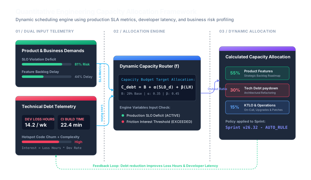
With these metrics established, we build a mathematical allocation model to determine the capacity split for the upcoming sprint. The engine acts as a closed-loop controller:

[Telemetry Inputs] -> [Capacity Router Engine] -> [Capacity Policy] -> [Sprint Execution] -> [Improved System Health] --(Feedback Loop)--> [Telemetry Inputs]

The target capacity for technical debt ($C_{debt}$) is computed dynamically using a baseline budget and scaling coefficients:

Where:

• $B$: The baseline capacity allocation (default is $15\%$). This is the minimum reserve required for routine package upgrades, vulnerability patches, and general maintenance.
• $\alpha$: Coefficient representing the sensitivity of capacity to production SLO breaches (typically set to $0.40$).
• $\beta$: Coefficient representing the sensitivity to developer developer loss hours ($0.30$).
• $\gamma$: Coefficient representing code risk profile ($0.30$).

The functions $f(x)$ map the metrics to a normalized scale between $0$ and $1$, representing the percentage of target capacity. We enforce an upper limit of $50\%$ for $C_{debt}$ to ensure product momentum does not stall completely, except in emergency scenarios where $SLOD > 0.8$, which triggers an immediate halt to all feature work to focus 100% of capacity on stabilization.

Here is a Python implementation of the evaluation logic:

def calculate_capacity_allocation(
    slo_deficit: float, 
    loss_hours_per_dev: float, 
    hotspot_count: int,
    team_size: int
) -> dict:
    # Configurations & Weights
    BASELINE = 0.15
    MAX_DEBT_CAPACITY = 0.50
    
    alpha = 0.40  # SLO weight
    beta = 0.35   # Loss Hours weight
    gamma = 0.25  # Hotspot weight
    
    # 1. Normalize SLO Deficit (0 to 1)
    # If deficit is greater than 5% of our error budget, we scale up rapidly
    norm_slo = min(1.0, slo_deficit / 0.05) if slo_deficit > 0 else 0.0
    
    # 2. Normalize Loss Hours
    # A team losing more than 15 hours per developer per month triggers maximum friction response
    norm_loss = min(1.0, loss_hours_per_dev / 15.0)
    
    # 3. Normalize Hotspot count
    # More than 5 high-risk hotspots in the repo triggers maximum focus
    norm_hotspots = min(1.0, hotspot_count / 5.0)
    
    # Calculate additional debt capacity
    additional_capacity = (alpha * norm_slo) + (beta * norm_loss) + (gamma * norm_hotspots)
    
    # Compute final values
    target_debt = min(MAX_DEBT_CAPACITY, BASELINE + additional_capacity)
    target_features = 1.0 - target_debt
    
    return {
        "technical_debt_capacity": round(target_debt, 2),
        "product_feature_capacity": round(target_features, 2)
    }

# Example run: High developer loss hours (12 hours) and active SLO breach
policy = calculate_capacity_allocation(
    slo_deficit=0.03, 
    loss_hours_per_dev=12.0, 
    hotspot_count=3,
    team_size=8
)
print(policy)
# Output: {'technical_debt_capacity': 0.45, 'product_feature_capacity': 0.55}

Translating Math into Sprint Execution

The output of this mathematical engine is a capacity allocation policy (e.g., 45% Tech Debt, 55% Product Features). To translate this into sprint execution without friction, the team must implement two key rules:

Automated Labeling and Ticket Sizing

All tickets in the sprint backlog must be labeled as either Product Feature (direct business value), Technical Debt (engineering health/refactoring), or KTLO (Keep The Lights On - e.g., security updates, on-call support).

During sprint planning, the total story points or hours committed must align with the calculated ratio. If the engine prescribes a 30% allocation for technical debt on a team with a velocity of 100 story points, exactly 30 points must be dedicated to tickets tagged with Technical Debt. The engineering leads are responsible for pulling the highest-ranked refactoring tasks from the backlog to fill this capacity.

Preventing Allocation Slippage

A common failure mode is “allocation slippage,” where engineers start working on product features during capacity designated for technical debt. To prevent this, the deployment pipeline should automate tracking.

For example, a GitHub Actions pre-merge hook can check that the proportion of Pull Requests tagged as technical debt matches the planned allocation within a $\pm5\%$ tolerance. If the team is falling behind their refactoring commitments, alert notifications are triggered, and product managers are prevented from scheduling additional feature releases.

Case Study: Dynamic Allocation in Action

Let’s look at how this framework functions in a real-world scenario. Consider an engineering team managing a high-frequency payment processing service. The service is written in Go and utilizes a PostgreSQL database.

Phase 1: Stable State

• Metrics: P99 latency is stable at $140\text{ms}$ (SLO target: $< 200\text{ms}$), CI/CD pipelines run in 5 minutes, code churn is low.
• Allocation: The engine outputs the baseline allocation:
  • Product Features: 85%
  • Technical Debt: 15%
• Outcome: The team focuses heavily on building out a new subscription billing module.

Phase 2: The Onset of Friction

• Metrics: The subscription billing module is rushed to production. The codebase grows complex; database locks begin to pile up under peak load due to nested transactions. CI/CD pipeline duration jumps to 22 minutes because the integration test suite grows bloated. Developer loss hours climb to 14 hours/week per developer.
• Allocation: The next iteration calculation inputs the degraded metrics:
  • $SLOD$: 0.02 (SLO availability drops slightly to 99.8%)
  • $LH$: 14 hours
  • Hotspot count: 4 complex files with high commits
  • Calculated Allocation:
    • Technical Debt: 45%
    • Product Features: 55%
• Outcome: The product manager is blocked from introducing three new feature stories. Instead, the team uses the 45% capacity to optimize the database query paths, introduce connection pooling via pgbouncer, split the integration test suite to run in parallel, and refactor the transaction control flow.

Phase 3: Recovery

• Metrics: After a single sprint under the 45% technical debt policy, the CI/CD pipeline time drops to 6 minutes. Connection contention disappears, and latency drops back to $120\text{ms}$. Developer loss hours fall back to 3 hours/week.
• Allocation: The engine processes the updated metrics:
  • Technical Debt: 20%
  • Product Features: 80%
• Outcome: The team resumes high-velocity feature development, having successfully cleared the structural debt before it could trigger a catastrophic production outage.

Pitfalls and Anti-Patterns of Quantitative Capacity

While a telemetry-driven capacity model eliminates negotiations and stabilizes codebases, engineering organizations must watch out for three critical anti-patterns when implementing it.

1. Metric Gaming

Once engineers realize that high cyclomatic complexity or long build times increase their technical debt budget, they may subconsciously (or consciously) alter their behavior. Developers might write bloated code to artificially inflate complexity, or write slow, unoptimized tests to increase CI runtimes.

To mitigate this, metrics must be audited regularly. The Code Hotspot Index, for example, should only count churn from files modified in merged pull requests that have passed peer review.

2. Over-Engineered Models

It is easy to get bogged down trying to design the “perfect” algorithm. Teams can waste weeks calibrating weights ($\alpha, \beta, \gamma$) to decimals, or integrating overly complex statistical models.

Start simple. A model that uses only two variables—CI pipeline duration and SLO error budget consumption—is often enough to capture 80% of the value. The goal is to build an objective, repeatable feedback loop, not a neural network.

3. Metric Detachment

The framework should never replace human common sense. If a critical architectural flaw exists that does not show up in telemetry—such as a deprecated third-party service dependency that will shut down next month—engineering leads must have the authority to override the model. The quantitative framework should act as a guardrail and a scheduler, not a rigid prison.

Conclusion

Engineering capacity is finite. When you manage it based on negotiation, loudest-voice politics, or arbitrary percentages, you compromise both the operational stability of your systems and the productivity of your developers.

By defining clear, measurable metrics for developer friction and system health, and processing them through a dynamic control loop, you treat technical debt as a real business cost. This framework removes emotion from the planning room, protects developer sanity, and ensures that product velocity is sustained not by cutting corners, but by maintaining a reliable, high-performance foundation.