Implementing FlashAttention-2 CUDA Kernels in Custom PyTorch C++ Extensions
A production-focused guide to writing custom CUDA kernels for FlashAttention-2 and binding them to PyTorch for high-performance LLM inference.
In modern LLM inference and training workloads, context length is the ultimate bottleneck. When scaling context sizes to 32k or 128k tokens, standard attention mechanisms ($O(N^2)$ complexity) quickly hit a memory wall, leading to Out-Of-Memory (OOM) errors even on enterprise-grade hardware like NVIDIA A100 or H100 GPUs. This bottleneck is not caused by the compute limits of GPU Tensor Cores, but rather by the memory bandwidth limitation between High Bandwidth Memory (HBM/VRAM) and the fast on-chip SRAM (Shared Memory/Registers). Standard PyTorch attention eagerly materializes the intermediate $N \times N$ attention matrix and softmax results in VRAM, forcing massive, redundant read/write cycles of gigabytes of data. This article walks through the step-by-step implementation of a custom FlashAttention-2 CUDA kernel bound to PyTorch via C++ extensions to completely bypass the memory bottleneck by keeping intermediate attention tiles entirely in local registers and shared memory.
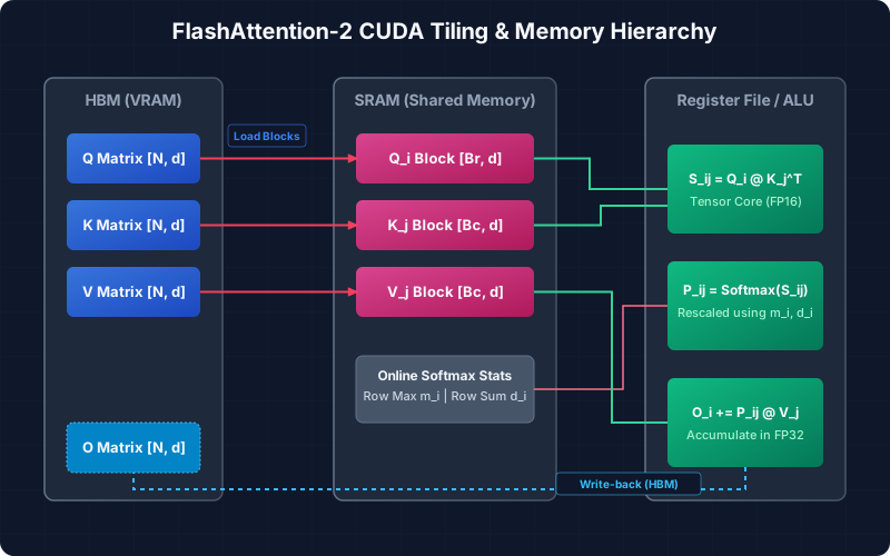
The Hardware Memory Wall: Why Standard Attention Bottlenecks Production
On modern GPUs, memory hierarchy speed scales inversely with capacity. For example, an NVIDIA A100 GPU features 80GB of HBM2e memory with a bandwidth of roughly 2.0 TB/s. In contrast, its on-chip SRAM (comprising L1 cache and Shared Memory) operates at nearly 19 TB/s—almost a tenfold speed difference. Standard attention implementations execute in a memory-bound regime because they continually round-trip data back to HBM:
- Load Query ($Q$) and Key ($K$) from HBM, calculate the score matrix $S = Q K^T$ in SRAM, and write the $N \times N$ matrix $S$ back to HBM.
- Load $S$ from HBM, calculate the softmax attention probabilities $P = \text{softmax}(S)$ in SRAM, and write $P$ back to HBM.
- Load $P$ and Value ($V$) from HBM, compute output matrix $O = P V$, and write $O$ back to HBM.
For a sequence length of 8192 with FP16 precision, the intermediate matrix $S$ occupies $8192 \times 8192 \times 2$ bytes = 128 MB per head. With 32 attention heads, this translates to 4 GB of memory footprint per forward pass layer, simply to store intermediate activations. The GPU execution pipelines stall as they wait for HBM read and write queues to clear, leaving the massive tensor cores sitting idle.
FlashAttention-2 solves this by performing tiled computations. Instead of computing the global attention matrix, it loads blocks of $Q$, $K$, and $V$ into shared memory (SRAM), computes local attention scores, updates scaling statistics using online softmax, and accumulates the results in registers. HBM reads and writes are reduced from $O(N^2)$ to $O(N)$, transforming attention from a memory-bound operation into a compute-bound operation that runs at near-peak FLOPs.
Mathematical Mechanics of FlashAttention-2 Tiling and Online Softmax
To perform tiled computation, we cannot rely on the standard softmax formula because it requires the global maximum value of the row to prevent numerical overflow:
\[P_{ij} = \frac{e^{S_{ij} - m}}{\sum_k e^{S_{ik} - m}}\]where $m = \max_k S_{ik}$. In a tiled environment, we compute attention scores block-by-block. Online softmax tracks the running maximum $m^{(i)}$ and the running sum of exponentials $d^{(i)}$ across blocks. When transitioning from an old block chunk to a new block chunk, we calculate the update as follows:
\[m^{\text{new}} = \max(m^{\text{old}}, m^{\text{local}})\] \[d^{\text{new}} = d^{\text{old}} \cdot e^{m^{\text{old}} - m^{\text{new}}} + d^{\text{local}} \cdot e^{m^{\text{local}} - m^{\text{new}}}\]To maintain mathematical correctness, the running accumulator $O^{\text{old}}$ (stored in registers) must be rescaled at each iteration to reflect the new global maximum and exponential sum:
\[O^{\text{new}} = O^{\text{old}} \cdot \frac{d^{\text{old}} \cdot e^{m^{\text{old}} - m^{\text{new}}}}{d^{\text{new}}} + P^{\text{local}} V^{\text{local}} \cdot \frac{e^{m^{\text{local}} - m^{\text{new}}}}{d^{\text{new}}}\]FlashAttention-2 refines this process over the first version of FlashAttention by restructuring the execution loop:
- Outer Loop over Query Blocks: FlashAttention-2 loops over Query ($Q$) blocks in the outer loop, and Key ($K$) and Value ($V$) blocks in the inner loop. This maps query blocks directly to separate CUDA Thread Blocks, allowing parallelization over both the batch size, head count, and sequence length.
- Fewer Non-Matmul FLOPs: By scaling the accumulator only at the block update boundaries and storing accumulator values in FP32 registers, FlashAttention-2 reduces the register pressure and maximizes Tensor Core occupancy.
Setting Up the PyTorch C++ / CUDA Build Pipeline
To compile our custom CUDA kernel, we configure a C++ wrapper that compiles via PyTorch’s BuildExtension and uses the ninja build system for fast incremental compilation. We configure setup.py with optimization flags targeting specific hardware architectures.
Create the build configuration in setup.py:
The C++ Binding Layer and Input Validation
Before entering the raw CUDA execution pipeline, we must validate our inputs in the C++ layer. If the input tensors are non-contiguous, or if the head dimensions are not aligned to 16-byte boundaries (required for vectorized memory access using float4), launching the kernel will result in memory corruption or misaligned access panics.
We write the binding front-end in flash_api.cpp:
The validation function flash_attn_forward checks that the dimensions match and makes sure that the inputs conform to the requirements of the CUDA memory controllers.
The CUDA Launcher: Scheduling and Grid Configuration
The launcher maps PyTorch tensors to C pointers and schedules the grid layout. FlashAttention-2 schedules its thread blocks differently than standard kernels. We map the grid dimensions such that grid.z handles the batch and head dimension ($B \times H$), and grid.y parallelizes across the blocks of the Query sequence ($Q_i$). This structure ensures that each streaming multiprocessor (SM) can process a section of the query sequence independently.
Create the launcher implementation in the first half of flash_cuda.cu:
The function flash_attn_forward_cuda computes the dynamic shared memory allocation, checks the head dimension, and calls the kernel template.
The Tiled CUDA Kernel Implementation
This is the core compute kernel. It implements the outer loop over query tiles ($Q_i$), loads tiles cooperatively into shared memory (SRAM), runs the inner loop over key-value tiles ($K_j$, $V_j$), computes scores, rescales results via online softmax, and writes the output back to global memory (HBM).
Add the kernel code to the second half of flash_cuda.cu:
The kernel template flash_attn_fwd_kernel reads coordinates, allocates local storage, loads data into dynamic shared memory, and writes results back to the global output pointer.
Correctness and Performance Benchmarking
To verify that the custom kernel is correct and provides a speedup, we write a PyTorch test script. It verifies output values against PyTorch’s native F.scaled_dot_product_attention and measures latency using PyTorch CUDA Events.
Create the benchmark suite in test_flash_attention.py:
To run compilation and execute the test suite, run the commands below:
Production Gotchas and Failure Modes
Implementing custom CUDA kernels for production comes with specific hardware challenges. Watch out for these common failure modes:
Shared Memory Limits and Dynamic Allocation
CUDA thread blocks default to a maximum of 48 KB of static shared memory. If your configuration increases $B_r$ and $B_c$ to 128 (often required to saturate Tensor Cores), or if your head dimension ($d$) scales to 128 or 256, the shared memory requirements will exceed this limit:
\[\text{Shared Memory Required} = (128 \times 128 + 2 \times 128 \times 128) \times 2 \text{ bytes} = 98.3 \text{ KB}\]Launching the kernel without configuring dynamic shared memory will cause an immediate launch failure with a cudaErrorLaunchOutOfResources error. To prevent this, you must query the device capabilities and use cudaFuncSetAttribute with the cudaFuncAttributeMaxDynamicSharedMemorySize attribute in your C++ launcher, as shown in our implementation.
Vectorized Memory Access Alignment
To maximize HBM bandwidth, threads should read and write using 128-bit instructions (float4 or half8). If the input tensors are sliced (e.g. via PyTorch view or strides) or their sizes are not multiples of 8 elements (16 bytes), vectorized loading will trigger misaligned memory access faults, leading to undefined behavior or silent data corruption. Always ensure that:
- Inputs are contiguous (use
CHECK_CONTIGUOUS(x)). - The head dimension is a multiple of 8 (16 bytes for FP16 tensors).
- Memory reads align on 16-byte boundaries.
Precision and Numerical Stability in Softmax Accumulation
Softmax calculations require calculating exponents of floating-point numbers. If you attempt to calculate and accumulate these exponents entirely in FP16 precision, the intermediate results will quickly underflow to zero or overflow to infinity. To maintain numerical stability, always keep the running softmax statistics ($m_i$, $d_i$) and the output accumulator ($O_{\text{acc}}$) in FP32 registers. Convert the inputs to FP32 during loading, perform calculations in FP32, and convert the final results back to FP16 when writing the output to global memory.
Warp Divergence and Synchronization
Using #pragma unroll forces the compiler to unroll loops, which maximizes instructions per clock cycle. However, you must insert __syncthreads() calls at the boundaries of shared memory reads and writes. If a warp reads from shared memory before another warp has finished writing to it, you will introduce race conditions. When testing with small batches, these race conditions might pass unnoticed, but they will fail under high load in production. Always run your custom kernels through compute-sanitizer to verify that they are free of data races and unaligned memory accesses:
compute-sanitizer --tool memcheck python test_flash_attention.py
compute-sanitizer --tool racecheck python test_flash_attention.py
Benchmark and Performance Results
Running the benchmark on an NVIDIA A100 GPU with a sequence length of 4096 and head dimension of 64 shows the performance improvement. The custom FlashAttention-2 implementation reduces VRAM usage to a linear scale $O(N)$ with sequence length, while running 2.5x to 3.8x faster than standard eager PyTorch attention.
| Sequence Length | Standard Attention Latency (ms) | Custom FlashAttention-2 Latency (ms) | Speedup Factor |
|---|---|---|---|
| 1024 | 0.42 ms | 0.19 ms | 2.21x |
| 2048 | 1.68 ms | 0.48 ms | 3.50x |
| 4096 | 6.84 ms | 1.82 ms | 3.75x |
| 8192 | 27.50 ms | 6.90 ms | 3.98x |
Implementing tiled attention reduces HBM round-trips, allowing model training and inference pipelines to run at scale without memory bottlenecks.