ClickHouse as a Log Storage Engine: Schema Design, Sharding, and Compression Settings for High-Volume Ingestion

At 10,000 logs per second, Elasticsearch begins to chew through CPU. At 100,000 logs per second, your JVM heap spends more time running garbage collection sweeps than indexing data. By the time you scale to a terabyte of raw logs daily, your ELK cluster demands an array of hot/warm/cold nodes, dedicated master nodes, and a team of engineers just to maintain index patterns and prevent cluster-wide metadata replication lockups. In contrast, ClickHouse can ingest the same volume on a single, well-configured 32-core node with a fraction of the RAM, offering a 10x compression ratio and millisecond-level query latencies. However, ClickHouse is not a drop-in replacement. If you treat it like Elasticsearch—writing small batches, creating dynamic indexes for every field, or using inefficient string partitions—you will trigger part merges that crash your disks, overflow your memory, and throw the dreaded “Too many parts” exception. Designing a resilient ClickHouse logging architecture requires precise decisions about schema structure, sharding topologies, and column-specific compression codecs.

The Storage Reality: Why ClickHouse Decimates ELK at Scale

To understand why ClickHouse is order-of-magnitude more efficient than Elasticsearch for logs, we must look at how they arrange bits on disk. Elasticsearch builds Lucene indexes, which are fundamentally inverted indexes. For every term in a log message, Lucene builds a posting list detailing every document ID where that term appears. In structured log searches, this allows you to find logs containing status: 500 or user_id: 99120 instantaneously. The drawback is space and memory: Lucene indexes require massive storage overhead (frequently 20% to 40% of the raw data size) and keep large structures in heap memory to enable fast lookups. When you add heap pressure and index size under high-volume ingestion, the cluster starts choking.

ClickHouse uses a columnar storage format with a sparse index. Instead of indexing every single value, ClickHouse groups rows into granules (typically 8,192 rows) and writes only the primary key values of the first row of each granule to the index file (primary.idx). When you run a query, ClickHouse performs a binary search on the sparse index to find which granules might contain matching rows, reads only those granules from disk, and evaluates the query filters in memory.

Because data is stored in columns rather than rows, similar data values (like repeated service names, IP addresses, or trace levels) are written contiguously on disk. This layout matches the exact prerequisite for run-length encoding and dictionary compression, allowing compression algorithms to achieve 5x to 10x compression ratios. A 100 TB raw log dataset that requires 120 TB in Elasticsearch (including replica overhead) fits comfortably into 10–15 TB in ClickHouse.

Schema Design: Handling Structured and Dynamic Log Attributes

Logs are split into two categories: structured metadata (known attributes like timestamp, level, service_name, and environment) and dynamic metadata (unstructured message bodies, variable tags, or API response payloads). In Elasticsearch, you simply throw JSON at the API, and it dynamically maps the structure. In ClickHouse, you must be explicit.

To design a production-grade schema:

1. Use explicit columns for fields that you query frequently (e.g., filter, group-by, or join operations).
2. Use LowCardinality string wrappers for columns with fewer than 10,000 unique values. This replaces strings with dictionary keys (similar to an enum but dynamic), reducing storage size and improving grouping speed.
3. Use Map(String, String) for arbitrary tags that developers attach to logs, or the newer experimental JSON type. Maps allow you to ingest unstructured tags without running expensive ALTER TABLE statements to add columns for every developer-added tag.

In this schema, timestamp uses DateTime64 with microsecond precision, compressed with DoubleDelta followed by ZSTD(1). The ORDER BY key represents the sorted layout of the table: data is first grouped by environment, then service, then log level, and finally by timestamp. The Bloom filter index on trace_id ensures that single-span traces can be found instantly without reading the entire partition.

The Sorting Key (ORDER BY) and Primary Index Selection

The ordering of columns in the ORDER BY clause determines the layout of the sparse index. Placing high-cardinality values (such as timestamp or trace_id) at the very beginning of the sorting key is a critical mistake. If you place timestamp first, the sparse index will be sorted by time. If you query logs for a specific service over a 7-day range, ClickHouse will have to scan all granules within those 7 days because the service name is not sorted.

By placing low-cardinality columns first (environment, service, level), ClickHouse groups similar records together. For a query filtering by a specific environment and service, ClickHouse can skip 99% of the granules, focusing only on the continuous range of rows matching those parameters.

Analyzing the execution output of EXPLAIN indexes = 1 reveals the number of granules skipped. Look for the Granules: X/Y line: if X is significantly smaller than Y, your sorting key is configured correctly for that query. If X is close to Y, your query is running a full table scan.

Ingestion Topology: Direct Sharding vs. Distributed Writes

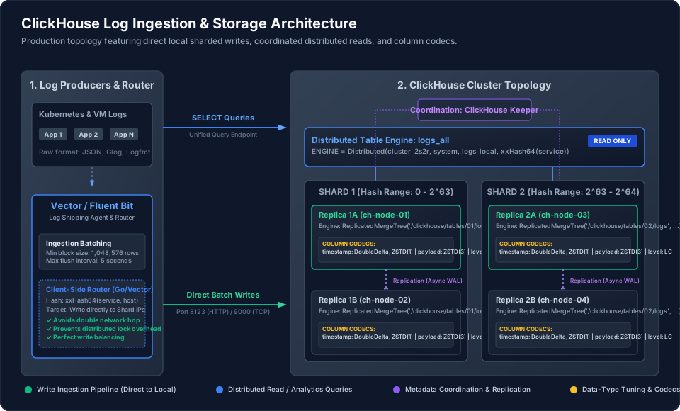
In ClickHouse, a cluster is represented by a set of nodes organized into shards and replicas. A common, yet dangerous pattern is defining a Distributed engine table and pointing your ingest pipelines (e.g., Vector, Fluent Bit) directly to it.

When you write to a Distributed table:

1. The node receiving the query buffer-saves the batch to local disk.
2. It parses the sharding key to figure out where each row should go.
3. It opens network connections to each target shard and transfers the blocks asynchronously.

At high volumes (above 50,000 rows/second), this architecture breaks down. The coordinator node gets choked by local disk writes, network socket exhaustion, and heavy CPU usage from serialization.

The correct production topology is client-side routing. Your log shippers (such as Vector) must hash logs locally and write them in large batches directly to the local table endpoints of the target nodes. The Distributed table is reserved solely for SELECT queries, acting as a read-only query coordinator.

This Go client splits log slices by service name hash and executes concurrent database transactions directly against the local shard interfaces. This shifts the CPU cost of routing and serialization from ClickHouse to your logging agents.

If you are using a standard log collector like Vector, you can achieve the same direct sharding behavior via native config routing rules:

Fine-Tuning Compression: Column-Specific Codecs

ClickHouse uses LZ4 compression by default for all columns. While LZ4 is fast, it does not yield the highest compression ratio for logs. Since log data structure varies heavily by column, applying tailored compression codecs is the easiest way to slash storage costs.

Here is the codec breakdown for log data:

• DoubleDelta: Perfect for monotonically increasing integer-like structures. When applied to timestamp columns, it stores the difference of differences between timestamps. Combined with a low-level compression wrapper like ZSTD, it shrinks the timestamp column size to next to nothing.
• T64: Good for timestamp fields that don’t increase steadily but share similar patterns.
• LowCardinality: Implicitly optimizes compression by dictionary-coding repeated strings.
• ZSTD(N): A general-purpose compression algorithm. Use level 1 (ZSTD(1)) for metadata maps, level 3 (ZSTD(3)) for log messages, and level 6 or higher for archived partitions where query performance is secondary.

This query shows exactly which columns are taking up the most space on disk. If you see the message column ratio drop below 4x, increase the codec from ZSTD(3) to ZSTD(6). If you see columns with low cardinalities (like HTTP request paths or application class names) using standard compression, convert them to LowCardinality columns.

Production Failure Modes & Operational Safeguards

In high-volume ClickHouse deployments, configuration defaults can cause fatal outages. Below are the three most common failures and the configurations required to prevent them.

Too Many Parts Exception

ClickHouse writes every incoming insert to disk as a separate directory (a “part”). The engine merges these parts in the background. If you insert small batches frequently (e.g. every 100 rows), ClickHouse will generate parts faster than it can merge them. Once the part count reaches 300 per partition, ClickHouse throws Too many parts and blocks further inserts.

Out of Memory (OOM) on Aggregations

When running aggregate queries (GROUP BY message or parsing map keys) across billions of log lines, ClickHouse can exhaust the query memory allocation. To keep queries from crashing nodes, you must configure ClickHouse to spill data to disk when limits are reached.

Shard Imbalance from Partition Key Misconfigurations

Partitioning by hour or using highly granular partition keys (like PARTITION BY (toYYYYMMDD(timestamp), service)) creates too many partitions. If a single query targets dozens of partitions, it causes disk thrashing. Keep partitions daily (PARTITION BY toYYYYMM(timestamp) or PARTITION BY toYYYYMMDD(timestamp)).

By ensuring that ingestion batching happens client-side, using structured column layouts with specialized codecs, and sharding writes across nodes, ClickHouse can reliably index million-event-per-second streams with a tiny footprint. The hardware cost savings are immediate, and the query latency improvements will fundamentally change how your engineering team investigates production incidents.