Aligning Architectural Refactors to Business Value: A Quantitative SLA-to-DORA Attribution Framework

Every senior engineering leader has faced the corporate dread of the “refactoring pitch”: attempting to convince a product manager or chief financial officer that rewriting a core payment ingestion loop or splitting a monolithic PostgreSQL instance is worth a two-month freeze on user-facing features. Product teams speak in terms of conversion rates, net promoter sales, and contract values; infrastructure teams counter with database connection pools, memory leaks, and thread saturation. When engineering fails to bridge this language barrier, one of two failures occurs: critical technical debt is ignored until a cascading outage wipes out three days of revenue, or a massive, multi-quarter “infrastructure modernization” project is greenlit with zero accountability, ending in a marginal performance boost that fails to justify its hundred-thousand-dollar developer-hour cost. To break this cycle, engineering organizations must move beyond qualitative hand-waving and implement a quantitative, telemetry-driven framework that mathematically attributes system performance shifts and DORA improvements directly to business financial value.

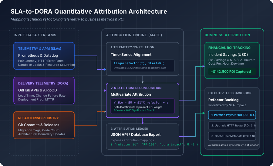
The Disconnection: Why Technical Excellence Fails to Justify Itself

In a production environment, technical debt does not exist in a vacuum. It manifests as slow execution paths, volatile database locking behavior, and brittle deployment pipelines. However, typical engineering metrics—specifically the four core DORA metrics (Deployment Frequency, Lead Time for Changes, Change Failure Rate, and Time to Restore Service)—often feel too abstract to business stakeholders. When you tell a Chief Financial Officer that your refactor of the checkout service improved Deployment Frequency from twice a week to four times a day, their immediate reaction is: So what? Did it drive more checkouts, or did it just allow us to deploy bugs faster?

Conversely, operational Service Level Agreements (SLAs) are often too coarse to guide architectural work. Traditional uptime SLAs (e.g., 99.9% availability) focus on absolute binary states—is the server returning a 200 OK or a 500 Internal Server Error? They fail to capture the degradation of user experience caused by long tail latencies. A service that is 100% “available” but suffers from a P99 latency of 4.2 seconds due to an $O(N)$ query in a nested Hibernate loop will drive users away just as effectively as a total outage.

To bridge this gap, we must establish a pipeline that maps code changes directly to operational telemetry, correlates that telemetry with SLA compliance, and translates the delta into business value.

The SLA-to-DORA Attribution Equation

To prove that an architectural change (like partitioning a database table or rewriting a legacy synchronous service in Go using concurrency primitives) caused a positive business outcome, we must isolate its impact. The core challenge is that production systems are highly dynamic. A drop in P99 latency following a deployment could be due to the refactor, but it could also be due to a concurrent drop in traffic volume, an automatic Kubernetes node scale-up, or a cache warm-up.

We can model the target Service Level Indicator (SLI) metric $Y_t$ (e.g., P99 response time in milliseconds) during an hourly window $t$ as a function of our refactoring deployment and key confounding variables:

Where:

• $X_{i,t}$ is a binary indicator variable representing the presence of refactor $i$ at time $t$. It is set to $0$ before the deployment and $1$ after the deployment.
• $Q_t$ represents the transaction throughput (requests per second) during hour $t$, controlling for load-based latency escalation.
• $H_t$ represents hardware capacity (e.g., active CPU cores, memory limits, database connection pool limits) at hour $t$.
• $\beta_i$ is the isolated attribution coefficient for refactor $i$. If $\beta_i$ is negative and statistically significant ($p < 0.05$), we have isolated a real performance improvement.
• $\epsilon_t$ is the residual error term, capturing unmeasured production noise.

We can apply a similar model to team velocity and DORA metrics. If we refactor a monolith into microservices, we expect our Lead Time for Changes (LTFC) to decrease. We isolate this change by comparing the commit-to-deploy duration of the affected service boundaries against control boundaries that did not undergo refactoring. The reduction in Change Failure Rate (CFR) directly translates to avoided incidents, which minimizes both developer interruption costs and SLA penalty payouts:

Where:

• $\Delta \text{CFR}$ is the percentage reduction in Change Failure Rate.
• $N_{\text{deploys}}$ is the annualized number of deployments.
• $\text{MTTR}$ is the Mean Time to Restore service in hours.
• $R_{\text{dev}}$ is the average hourly developer billing rate.
• $W_{\text{dev}}$ is the number of engineers pulled into a typical incident response call.
• $C_{\text{sla}}$ is the average hourly SLA credit payout or contract penalty cost during an outage.

Building the Data Pipeline: Telemetry and Event Ingestion

Implementing this attribution framework requires integrating two distinct data domains: deployment metadata and real-time operational telemetry.

1. The Architectural Ledger

First, we must capture every architectural change as a structured event. We configure a GitHub Action or an ArgoCD webhook to post a payload to our attribution engine’s ledger database every time a deploy occurs.

{
  "event_type": "deployment",
  "service": "payment-processor",
  "refactor_id": "RF-2026-08",
  "commit_sha": "d3b07384d113edec49eaa6238ad5ff00",
  "deployed_at": "2026-07-21T08:00:00Z",
  "scope": {
    "type": "database_partitioning",
    "target_table": "transaction_ledger",
    "migrated_records": 45000000
  }
}

2. Operational Telemetry Ingestion

Second, we pull metrics from our monitoring infrastructure. We leverage the OpenTelemetry (OTel) Collector to write metrics to a time-series store (such as Prometheus or TimescaleDB). Specifically, we ingest the following telemetry on a minute-by-minute basis:

• http_server_duration_milliseconds_bucket: To calculate P95 and P99 latencies.
• http_server_requests_total: To track throughput (RPS) and error rates.
• container_cpu_usage_seconds_total: To calculate CPU utilization.
• pg_stat_database_locks: To identify contention bottlenecks in PostgreSQL.

We run a scheduled worker that queries Prometheus via its HTTP API and aggregates this data into hourly buckets, aligning it with our deployment ledger timestamps.

# Querying Prometheus API for P99 latency of the payment-processor service
curl -G "http://prometheus.production.local/api/v1/query_range" \
  --data-urlencode "query=histogram_quantile(0.99, sum(rate(http_server_duration_milliseconds_bucket{service=\"payment-processor\"}[1h])) by (le))" \
  --data-urlencode "start=2026-07-20T08:00:00Z" \
  --data-urlencode "end=2026-07-21T08:00:00Z" \
  --data-urlencode "step=1h"

Isolating the Signal: Dealing with Confounding Variables in Production

A major pitfall of quantitative evaluation is correlation-causation confusion. If you deploy a database index cleanup at 2:00 AM on Sunday, latency will drop simply because user traffic is at its weekly minimum. If you compare Sunday’s latency against Saturday afternoon’s traffic peak, your metric is useless.

To eliminate this noise, our framework employs three techniques:

1. Traffic Normalization Curves

Instead of measuring raw latency, we map latency as a function of throughput. In database-bound applications, latency behaves non-linearly under load due to queueing theory (specifically Kendall’s notation and the Kingman formula). We train a baseline model of latency against throughput on pre-deployment data. Post-deployment, we measure the deviation of actual latency from this baseline model under equivalent traffic loads.

2. Difference-in-Differences (DiD) Analysis

When a global network fluctuation or cloud provider incident occurs, it degrades performance across all services. To isolate the refactor’s impact, we select a control service—a highly related microservice that did not receive the refactor but shares the same infrastructure (e.g., runs on the same Kubernetes node group and talks to the same database cluster).

We compute the difference between the target service and the control service before the deploy, and compare it to the difference after the deploy:

By subtracting the control service’s delta, we strip away environment-wide confounding noise.

3. Traffic Splitting (Canary Deployments)

The gold standard for attribution is route-splitting via a service mesh (such as Istio or Linkerd). When deploying the refactored code, we split traffic 50/50 between the legacy instance (Subset A) and the refactored instance (Subset B). Both subsets run concurrently, experiencing identical network noise, database state, and traffic spikes.

We measure the P99 latency and error rates of Subset A vs. Subset B over a 48-hour window. Since all external variables are identical, any delta in performance is directly attributable to the refactoring code.

Step-by-Step Implementation of the Attribution Engine

Here is a concrete implementation of our attribution engine. This Python script uses pandas and statsmodels to load aligned telemetry, build the design matrix, perform ordinary least squares (OLS) regression to isolate the refactor impact, and verify statistical significance.

import numpy as np
import pandas as pd
import statsmodels.api as sm

def analyze_refactor_impact(telemetry_csv_path: str, deploy_timestamp: str):
    """
    Analyzes the impact of a refactor deployment on service latency,
    isolating throughput and CPU utilization as confounding variables.
    """
    # 1. Load telemetry data (hourly intervals)
    df = pd.read_csv(telemetry_csv_path)
    df['timestamp'] = pd.to_datetime(df['timestamp'])
    df = df.set_index('timestamp').sort_index()
    
    # 2. Define the intervention variable (0 before deployment, 1 after)
    deploy_dt = pd.to_datetime(deploy_timestamp)
    df['is_refactored'] = (df.index >= deploy_dt).astype(int)
    
    # 3. Handle missing data by interpolation
    df = df.interpolate(method='time')
    
    # Target variable: P99 latency (ms)
    Y = df['p99_latency']
    
    # Predictors: Refactoring flag + Confounding variables (RPS and CPU)
    # We include a constant (intercept) for baseline latency
    X = df[['is_refactored', 'requests_per_second', 'cpu_utilization_percent']]
    X = sm.add_constant(X)
    
    # 4. Fit the Ordinary Least Squares (OLS) regression model
    model = sm.OLS(Y, X).fit()
    
    # 5. Extract metrics
    beta_refactor = model.params['is_refactored']
    p_value = model.pvalues['is_refactored']
    confidence_interval = model.conf_int().loc['is_refactored']
    r_squared = model.rsquared
    
    print("=== SLA-to-DORA Attribution Engine Analysis ===")
    print(f"Dataset Range: {df.index.min()} to {df.index.max()}")
    print(f"Deployment Time: {deploy_dt}")
    print(f"Model R-squared: {r_squared:.4f}")
    print("-" * 50)
    
    if p_value < 0.05:
        print(f"RESULT: SUCCESS (Statistically Significant, p = {p_value:.6f})")
        print(f"Isolated Latency Delta: {beta_refactor:.2f} ms")
        print(f"95% Confidence Interval: [{confidence_interval[0]:.2f} ms, {confidence_interval[1]:.2f} ms]")
        
        # Calculate percentage improvement against pre-deployment baseline
        pre_deploy_mean = df.loc[df.index < deploy_dt, 'p99_latency'].mean()
        pct_improvement = (-beta_refactor / pre_deploy_mean) * 100
        print(f"Pre-deploy Baseline P99 Latency: {pre_deploy_mean:.2f} ms")
        print(f"Isolated Performance Improvement: {pct_improvement:.1f}%")
    else:
        print(f"RESULT: INCONCLUSIVE (Not Significant, p = {p_value:.6f})")
        print("The refactor did not produce a statistically significant change in latency.")
        print(f"Estimated coefficient: {beta_refactor:.2f} ms (p-value indicates high probability of noise)")
        
    return model

# Example Usage:
# analyze_refactor_impact('payment_service_telemetry.csv', '2026-07-21T08:00:00Z')

Translating Telemetry into Financial ROI

Once we have isolated the delta ($\beta_i$) using our regression model, we translate it into dollars. We focus on three direct cost centers: compute resource reduction, avoided SLA payouts, and developer velocity gains.

Case Study: Partitioning a Hot Postgres Table

Let’s apply the framework to a real-world scenario. The payment team partitioned a massive transaction table that was suffering from lock escalation and slow index scans.

Service: payment-processor
Refactor: Range partitioning on 'created_at' and indexing 'user_id'
Duration: 3 weeks of developer time (2 Senior Engineers = $18,000 developer cost)

1. Compute Savings

Before the refactor, the database ran on a AWS RDS db.r6g.8xlarge instance (32 vCPUs, 256 GB RAM) to handle peak write contention and large index scans. The instance cost was $3.84 per hour.

Post-refactor, the OLS regression model showed that CPU utilization dropped by 45% under identical peak throughput. This allowed the infrastructure team to downscale the instance to a db.r6g.4xlarge (16 vCPUs, 128 GB RAM) costing $1.92 per hour.

2. Avoided SLA Penalties

Our enterprise client contracts guarantee that our API will respond within 500ms for 99% of requests. If we breach this SLA for a cumulative total of more than 15 minutes in a billing cycle, we owe a 10% contract refund. In the six months prior to the partition refactor, database locks caused 4 distinct incidents where latency spiked past the SLA threshold for a combined total of 42 minutes, costing the company $45,000 in refunds.

Following the refactor, table locks dropped to zero. Our attribution engine confirmed that the probability of breaching the 500ms SLA during peak hours dropped from 3.2% to 0.05%.

3. DORA CFR Interruption Recovery

The database fragility resulted in a high Change Failure Rate (CFR) of 8% on code deployments because minor migrations regularly timed out under load. Every migration failure required rollbacks, pulling 3 engineers into a war room. The mean time to restore (MTTR) was 3 hours.

Post-refactor, the partition architecture allowed schema changes to target localized tables, dropping the CFR to 1%.

Total ROI Summary

• Total Annual Savings: $114,379.20
• One-time Engineering Capital Cost: $18,000.00
• Payback Period: ~1.9 months
• Net Present Value (NPV over 3 years at 10% discount rate): $266,275.00

With these numbers in hand, the conversation with business leaders changes. You are no longer asking for time to “clean up the code”; you are presenting a business case with a 2-month payback period.

Operationalizing the Framework: The Executive Feedback Loop

Calculating these numbers after a refactor is valuable, but the real power of the SLA-to-DORA framework is realized when it is built into the planning lifecycle.

1. The Quantitative Backlog: Instead of sorting technical debt by developer frustration, sort it by projected financial impact. If a refactor targets a service that is currently driving SLA breaches, its prioritization coefficient increases.
2. Telemetry-Driven Retrospectives: Every major architectural release should trigger an automated report from the attribution engine. If the regression model shows $p > 0.05$ (meaning no statistical change occurred), the engineering team must investigate why their architectural model failed to deliver the expected system behavior. This prevents developers from falling into the trap of writing complex, over-engineered systems that add no real operational value.
3. Cross-Functional Trust: When business stakeholders see that engineering is accountable for its performance claims, they are far more willing to allocate resources to infrastructure work. Technical debt stops being a black hole of developer resources and becomes a predictable, high-yield investment vehicle.